Data-Driven Information-Theoretic Causal Bounds under Unmeasured Confounding

A practical way to bound causal effects without instruments, bounded outcomes, or sensitivity parameters.

• Paper (PDF): https://yonghanjung.me/assets/pdf/R_19.pdf
• Code: https://github.com/yonghanjung/Information-Theretic-Bounds

TL;DR

• Unmeasured confounding breaks point identification, but we can still produce valid and tight causal intervals.
• We derive data-driven f-divergence bounds from the propensity score alone.
• The framework handles unbounded outcomes and conditional effects without full SCM modeling.
• A debiased, Neyman-orthogonal estimator yields stable inference with ML nuisances.
• Synthetic and IHDP results show coverage across propensity regimes and tighter widths as n grows.

High-level critique: why partial identification still stalls in practice

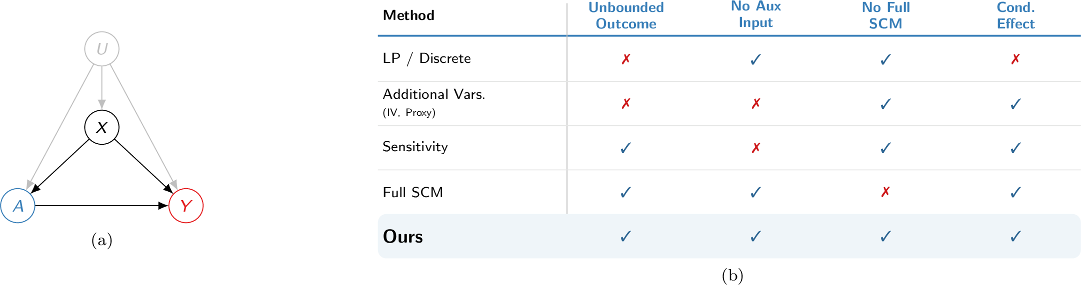
Problem setting with unmeasured confounding (left) and a positioning map of partial-ID approaches vs. our contribution (right).

Existing partial identification methods tend to trade away realism for tractability. Bounded outcomes make intervals look clean but collapse on heavy-tailed data. Auxiliary inputs such as IVs, proxies, or sensitivity parameters are powerful but often unavailable or not identifiable. Full SCM learning is expressive but brittle and computationally heavy. Most critically, many approaches stop at population averages and miss heterogeneity. The field needs a data-driven, model-light route to conditional causal bounds that remains valid with unbounded outcomes.

Formal justification: the bound that powers the story

We use the f-divergence, a generalized measure of discrepancy between probability distributions, to quantify the shift between the observational laws $P_{a,x}$ (where treatment $A=a$ is observed) and the interventional laws $Q_{a,x}$ (where treatment $A=a$ is forced). This naturally handles unbounded support by focusing on density ratios rather than absolute bounds on outcomes.

The central result links the unidentifiable interventional law to the identifiable observational law through a data-driven divergence radius:

\[D_f(P_{a,x} \| Q_{a,x}) \le B_f(e_a(x)) \equiv e_a(x) f\left(\frac{1}{e_a(x)}\right) + (1-e_a(x)) f(0).\]

This yields a distributionally robust ambiguity set around $P_{a,x}$, and the causal bound follows from a convex dual:

\[\theta_{\mathrm{up}}(a,x) = \inf_{\lambda>0, u} \Big\{ \lambda B_f(e_a(x)) + u + \lambda \, \mathbb{E}_{P_{a,x}}\big[g^{\ast}((\varphi(Y)-u)/\lambda)\big] \Big\}.\]

The dependence on $e_a(x)$ makes the bound fully data-driven, while the dual turns an infinite-dimensional optimization into a tractable problem.

Finally,

Method in one picture

flowchart LR
  subgraph Data-Driven Inputs
    obs["Data: P(X,A,Y)"] --> ps["Propensity: e(x)"]
    ps --> rad["Radius: B(e(x))"]
  end
  subgraph Robust Estimation
    rad --> amb["Ambiguity set: Q around P"]
    amb --> dual["Dual optimization (ƛ, u)"]
    dual --> est["Debiased estimator + k-agg"]
    est --> out["Causal interval: [Lower, Upper]"]
  end

Results: what the plots show

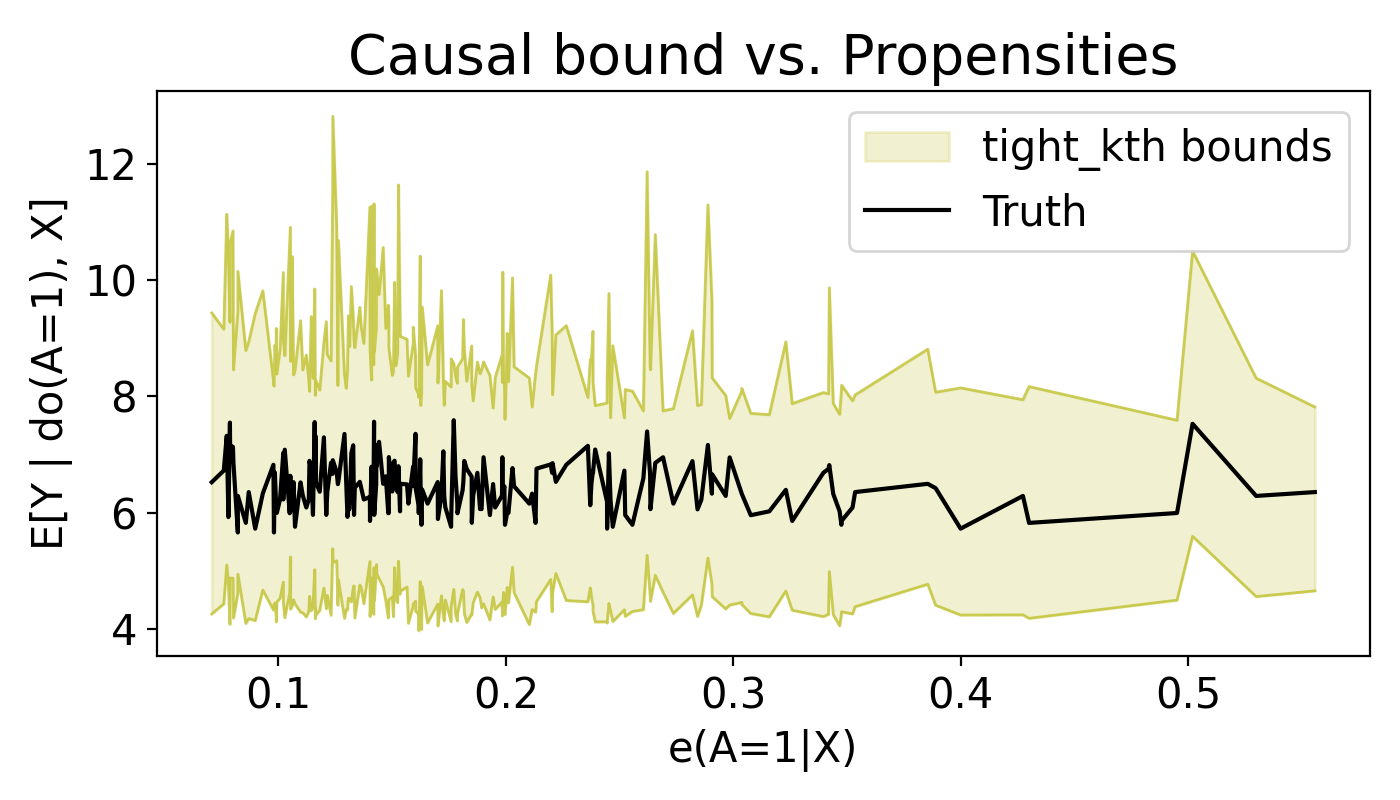
Quick note on tight_kth (the label used in the plots): we employ an order-statistics aggregator (Def. 7 in the paper) that computes candidate intervals from multiple f-divergences (KL, Jensen-Shannon, Hellinger, TV, $\chi^2$) and selects the $k$-th tightest valid bound. This method provides robustness against finite-sample instability where a single divergence might under-cover, ensuring that the final interval remains valid as long as at least $n_f - k + 1$ divergences are reliable.

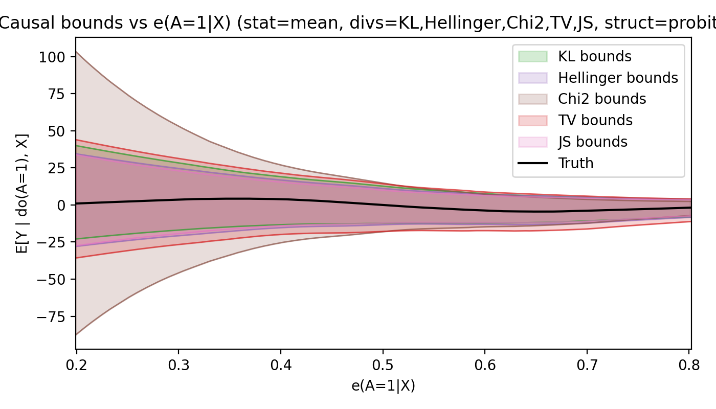
Synthetic: heavy tails with valid coverage

We simulate heavy-tailed outcomes (t with 3 df). The true conditional effect curve stays inside the estimated interval across all propensity regimes. As overlap improves, the bounds tighten exactly as the theory predicts.

Debiasing tightens intervals as n grows

Debiasing reduces penalized width and preserves convergence when propensity estimation is noisy. The orthogonal construction is doing real work here.

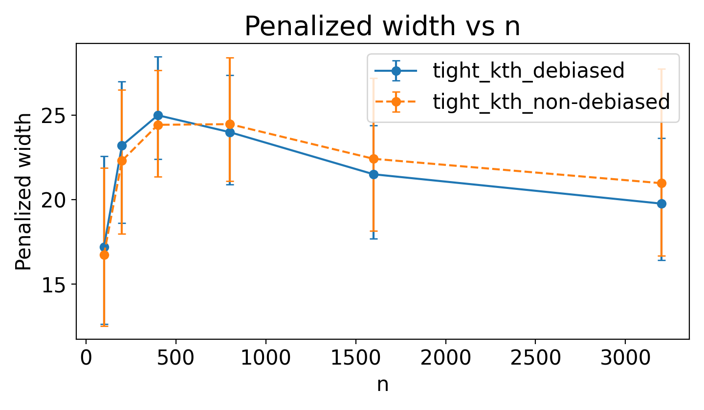Penalized width vs n.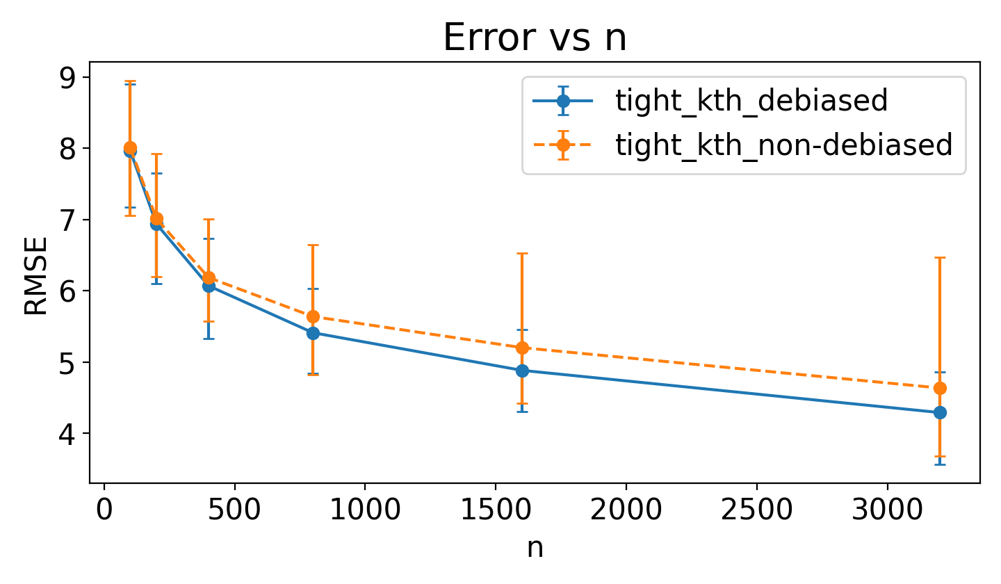

RMSE vs n under noisy propensity.

Fig. above (left) compares penalized width, a compound metric defined as $\text{p-width} \triangleq \mathrm{width} \times (1+ 10 \times \max (0, 0.05-\mathrm{coverage}))$. This metric heavily penalizes intervals that fail to cover the true effect (target 95%), forcing a trade-off where simple narrowness is not rewarded if validity is sacrificed. As shown, the debiased estimator achieves significantly tighter penalized widths as sample size increases, confirming its superior finite-sample efficiency.

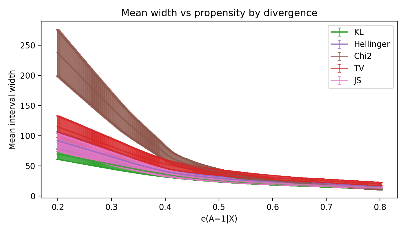
Propensity sweep: tighter bounds at higher overlap

This view makes the data-driven nature of the bound tangible. Higher propensity means smaller divergence radius and narrower intervals.

IHDP benchmark: realistic confounding

On the semi-synthetic IHDP benchmark with hidden confounders, the bounds tightly contain the true effect across the full range of estimated propensity scores.

Practical takeaways for applied users

• You can bound conditional effects without instruments, proxies, or sensitivity parameters.
• Unbounded outcomes are allowed, which matters for heavy-tailed data.
• Use multiple divergences and the k-aggregator to guard against finite-sample instability.
• ML models for the propensity and dual parameters are safe when debiased with orthogonality.

If you only read one thing

The whole framework turns a single learned propensity score into tight, data-driven causal intervals. It is a rare combination: identification without external inputs, robustness to heavy tails, and conditional effects that remain computationally feasible.