Heterogeneous Front‑Door Effects, Gently Explained
This is a gentle introduction of our work, accepted to ICLR 2026, on estimating heterogeneous Front‑Door Effects.
TL;DR. When unmeasured confounding breaks back‑door adjustment but a mediator is observed and well‑explained by covariates, front‑door adjustment can still identify causal effects. This post introduces two learners—FD‑DR‑Learner and FD‑R‑Learner—that estimate heterogeneous (personalized) front‑door effects. FD-DR satisfies a product-error bound, and FD-R satisfies a stage-error decomposition built from two back-door R-learner subproblems plus a final pseudo-$g$ regression. These results give conditional quasi-oracle guarantees when the nuisance remainders are no larger than the relevant oracle terms. We summarize the ideas, give intuition, show when to use which method, and point you to code.
What “debiased” and “quasi‑oracle” mean here
-
Debiased / orthogonal: the loss functions are constructed so that first-order nuisance errors are reduced or removed under the stated sample-splitting, overlap, moment, and stage-learning assumptions. Remaining error is tracked through product-error terms or named stage remainders.
-
Conditional quasi-oracle rate: An oracle rate is the achievable rate for the target parameter when the relevant nuisance or stage functions are given. A quasi-oracle interpretation is justified when the estimated-nuisance remainder is lower order than that oracle term.
- 0) Quick links
- 1) Why front‑door HTE?
- 2) Setup & notation (all symbols defined up front)
- 3) Two debiased learners at a glance
- 4) FD‑DR‑Learner — idea, pseudo‑outcome, and steps
- 5) FD‑R‑Learner — decomposition, pseudo‑g, and steps
- 6) Snippets on Main Result
- 7) Which learner should I use?
- 8) Practical checklist
- 9) Minimal “how-to” with the code
- References
0) Quick links
- Paper (ICLR 2026 accepted; tech report) — Debiased Front-Door Learners for Heterogeneous Effects
- Code — https://github.com/yonghanjung/FD-CATE (reproducible experiments and learners).
1) Why front‑door HTE?
With observational data, unmeasured confounding often prevents identification of causal effects via the usual back‑door (ignorability) route. Front‑door (FD) adjustment, introduced by Pearl [1], saves the day when a mediator $Z$ carries the effect from treatment $X$ to outcome $Y$, and $Z$ is “sufficiently” explained by observed covariates $C$. Many FD estimators target average treatment effects. However, in practice, we need personalized effects $\tau(C)$ per unit’s baseline characteristics $C$. This work fills that gap with debiased, ML‑friendly HTE estimators under FD.
2) Setup & notation (all symbols defined up front)
- Observed data: $V=(C,X,Z,Y)$, i.i.d.
- $C$: covariates (vector).
- $X\in {0,1}$: binary treatment.
- $Z\in {0,1}$: binary mediator.
- $Y$: outcome (real-valued).
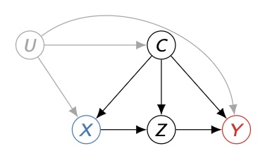
- $U$: unobserved confounders (affecting $C,X,Y$).
- Nuisance functions (all conditional on $C=c$ unless noted):
- Outcome regression: $m(z,x,c)\triangleq \mathbb{E}[Y\mid Z=z, X=x, C=c]$.
- Propensity for treatment: $e(x\mid c)\triangleq \Pr(X=x\mid C=c)$; write $e_1(c)=e(1\mid c)$, $e_0(c)=1-e_1(c)$.
- Mediator mechanism: $q(z\mid x,c)\triangleq \Pr(Z=z\mid X=x,C=c)$.
-
Target (CATE under FD):
\[\tau(C)\triangleq \mathbb{E}[Y\mid do(X{=}1),C]-\mathbb{E}[Y\mid do(X{=}0),C].\]Under the FD criterion (stated next), this equals
\[\tau(C)=\sum_{z,x}\big\{q(z\mid 1,C)-q(z\mid 0,C)\big\}e(x\mid C)\,m(z,x,C).\](This is Eq. (4) in the paper.)
-
Front-door criterion (intuitive):
- All causal paths $X\to Y$ go through $Z$ (no unmediated direct effect).
- Spurious paths $X\leftrightarrow Z$ are blocked by $C$.
- Spurious paths $Z\leftrightarrow Y$ are blocked by $(X,C)$.
3) Two debiased learners at a glance
We provide two estimators for $\tau(C)$
(1) FD-DR-Learner Builds a pseudo-outcome whose conditional mean equals $\tau(C)$ at the true front-door nuisances and regresses the estimated pseudo-outcome difference on $C$. Its error is controlled by a final target-regression term plus the conditional FDPO bias term $B_1-B_0$.
(2) FD-R-Learner Uses a partial linear decomposition of the FD system (two BD-R subproblems for $X\to Z$ and $Z \to Y$), plus a pseudo-g construction to remove first-order dependence on the treatment propensity in the final conditional average. Its theorem is a stage-error decomposition, and quasi-oracle behavior follows only when the BD-R and final-stage nuisance leakages are lower order.
4) FD‑DR‑Learner — idea, pseudo‑outcome, and steps
Weights and induced functionals. Define
\[\xi_{\bar x}(Z,X,C)\equiv \frac{q(Z\mid \bar x,C)}{q(Z\mid X,C)},\qquad \pi_{\bar x}(X,C)\equiv \frac{\mathbb{I}\{X=\bar x\}}{e(X\mid C)}.\] \[r_{m,e}(Z,C)\equiv \sum_x m(Z,x,C)e(x\mid C),\quad \nu_{m,e,q}(X,C)\equiv \sum_z r_{m,e}(z,C)q(z\mid X,C),\] \[s^{\bar x}_{m,q}(X,C)\equiv \sum_z m(z,X,C)\,q(z\mid \bar x,C).\]Front-door pseudo-outcome (FDPO).
\[\phi_{\bar x}(V;\eta)=\xi_{\bar x}\{Y-m\}+\pi_{\bar x}\{r_{m,e}-\nu_{m,e,q}\}+s^{\bar x}_{m,q}.\]Key property at the true nuisances: $\mathbb{E}[\phi_{\bar x}(V;\eta_0)\mid C]=\mathbb{E}[Y\mid do(X{=}\bar x),C]$, so
\[\mathbb{E}[\phi_1(V;\eta_0)-\phi_0(V;\eta_0) \mid C] = \tau(C).\]With estimated nuisances, the theorem separates the final regression error from the conditional FDPO bias $B_1-B_0$. We use “double robustness” in this product-error sense: the bound improves when the relevant nuisance products are small, rather than claiming that arbitrary misspecification of one nuisance block is harmless.
Algorithm (two-way cross-fit).
- Split data into $D_1,D_2$.
- On $D_1$: fit $\hat m,\hat e,\hat q$.
- On $D_2$: compute $\hat\phi_1-\hat\phi_0$ and regress it on $C$ (any ML regressor + regularization) to get $\hat\tau_{DR}(C)$.
- Swap folds and average.
Pros/cons. FD-DR is robust to nuisance misspecification and straightforward to implement. It uses inverse weights/density ratios $\pi_{\bar x},\xi_{\bar x}$, which can inflate variance when overlap is weak (propensities near 0 or 1).
5) FD‑R‑Learner — decomposition, pseudo‑g, and steps
Partial linear view of FD. Under the FD criterion the system can be written as
\[\begin{aligned} X&=e_X(C)+\varepsilon_X, \\ Z&=a(C)+X\,b(C)+\varepsilon_Z, \\ Y&=f(X,C)+Z\,g(X,C)+\varepsilon_Y, \end{aligned}\]with appropriate mean-zero conditions. The heterogeneous effect factorizes as
\[\tau(C)=b(C)\,\gamma_g(C),\qquad \text{ where } \quad \gamma_g(C)\triangleq \mathbb{E}[g(X,C)\mid C].\]Estimating $b$ and $g$ via BD-R.
- Treat $(Z,X,C)$ as an R-learner setup to learn $b(C)$.
- Treat $(Y,Z,(X,C))$ as an R-learner setup to learn $g(X,C)$.
The final theorem keeps the two BD-R oracle-plus-nuisance decompositions explicit as $R_b+N_b$ and $R_g+N_g$.
The pseudo-g trick. A naive plug-in for $\gamma_g(C)$ depends linearly on the error in $e_X$. Instead define
\[\zeta(X,C)=\big(1-\tilde e_X(C)\big)\tilde g(0,C)+\tilde e_X(C)\tilde g(1,C) +\{X-\tilde e_X(C)\}\{\tilde g(1,C)-\tilde g(0,C)\}.\]Then the conditional bias of $\zeta$ has no first-order term in $\tilde e_X-e_X$; it is driven by the quality of $\tilde g$ (Lemma 3). Regress $\zeta$ on $C$ to get $\hat\gamma(C)$. Finally, set $\hat\tau_R(C)=\hat b(C)\hat\gamma(C)$. (Def. 5, Thm. 3.)
Algorithm (three-way cross-fit).
- Split into $D_1,D_2,D_3$.
- On $D_1$: fit nuisances $e_X,m_Z,e_Z,m_Y$.
- On $D_2$: run BD-R to learn $\hat b(C)$ and $\hat g(X,C)$.
- On $D_3$: build $\hat\zeta$ and regress on $C$ to get $\hat\gamma(C)$.
- Output $\hat\tau_R(C)=\hat b(C)\hat\gamma(C)$.
- Swap folds and average.
Pros/cons. FD-R avoids density ratios (good under weak overlap) and yields interpretable pathway components $\hat b,\hat g$. It requires more nuisance fits than FD-DR. See §4.1.
6) Snippets on Main Result
The main theorems show how the two learners control nuisance error under front-door identification. FD-DR decomposes the error into a final target-regression term and a conditional FDPO bias term. FD-R decomposes the error into oracle stage errors and nuisance leakages: $R_b+N_b$ and $R_g+N_g$ are the two BD-R subproblem decompositions, while $R_\gamma+N_\gamma$ belongs to the final pseudo-$g$ regression.
The quasi-oracle message is conditional. If the FD-DR conditional bias is lower order than the final target-regression oracle rate, FD-DR has the same first-order rate as that oracle. If the FD-R nuisance leakages $N_b+N_g+N_\gamma$ are lower order than the oracle stage terms $R_b+R_g+R_\gamma$, FD-R has the same first-order rate as the oracle stage decomposition.
Theorem 3 is therefore a stage-error decomposition, not a standalone fast-rate theorem. It becomes a fast-rate or quasi-oracle statement only after one supplies separate rate bounds showing that the BD-R and final-regression nuisance remainders do not dominate the oracle terms.
7) Which learner should I use?
-
Use FD-DR-Learner when FDPO nuisance products can be controlled and overlap diagnostics are stable. You benefit from the product-error debiasing structure, but inverse weights can raise variance when overlap is weak.
-
Use FD-R-Learner when avoiding density ratios or inspecting the $X\to Z$ and $Z\to Y$ pathway components matters. Its formal guarantees still require the stated assumptions and stage-error conditions.
This mirrors the analytical comparison in §4.1 and the patterns in Fig. 2.
8) Practical checklist
-
Positivity/overlap diagnostics. Check empirical support of $e(X\mid C)$ and $q(Z\mid X,C)$; consider ratio stabilization/weight clipping (on denominators only) and overlap-aware uncertainty. (See discussion & limitations.)
-
Cross-fitting. Always split to avoid overfitting-induced bias.
-
Modeling choices. Any ML works; in our experiments we used XGBoost with small trees and ridge on the final regression. Hyperparameters aren’t delicate here; the orthogonalization carries a lot of the weight.
-
Diagnostics. Inspect $\hat b(C)$ (how law changes belt use) and $\hat g(X,C)$ (how belt use changes fatalities given $X,C$); probe SHAP/feature importances to understand heterogeneity.
9) Minimal “how-to” with the code
The repository contains scripts to reproduce the synthetic and FARS analyses. In particular, the supplement references a script named analyze_fars_2000_fd.py for the state seat-belt case study; use it as a template for your own data pipeline.
Generic workflow:
- Prepare your data frame with columns $C, X, Z, Y$ (binary $X,Z$ for the current theory).
- Choose a learner (FD-DR or FD-R) and ML backends for nuisances ($m,e,q$ or $e_X,m_Z,e_Z,m_Y$).
- Enable cross-fitting (2-fold for FD-DR, 3-fold for FD-R) and fit.
- Plot $\hat\tau(C)$, summarize by subgroups, and run overlap/weight diagnostics.
(See the repo’s README/examples; keep nuisance models simple and stable—orthogonalization will do its job.)
References
[1] Judea Pearl. Causality: Models, Reasoning, and Inference. 2nd ed., Cambridge University Press, 2009.